Operations Research: A Supply Chain Perspective Part 2
Last month, we introduced operations research (OR) and discussed how its methodology is applied to assist us in finding feasible or optimal solutions to supply chain problems. The role of the OR model continues to pervade supply chain operations, and this has stimulated a wealth of decision tools available to the market. These tools are used by practitioners to model and optimise transport routes, fleet profiles, inventory allocations, DC locations, manufacturing schedules, and so on.
Interestingly, most commercial software systems available today seldom use proprietary formulations. Quite often, algorithms are based on traditional programming techniques, while conventional heuristics are used by the most popular packages. On the other hand, most commercial platforms offer sufficient scalability, and many have attractive user-interface features.
Continuing our series on OR in the supply chain, we now look at the Assignment Problem and show how it can be used to decide on work and resource allocations. To illustrate, we examine one of our recent case studies involving the configuration of resources in an eCommerce fulfillment operation, and in order to demonstrate this integer-type formulation, we treat this problem using Microsoft’s Solver© add-in (note: although this module is limited in decision variables and constraints, it can nevertheless be used in this small-scale example).
The Assignment Problem
Is actually a special case of the Transportation Problem (see last month’s article) in which a number of resources (e.g. operators) are assigned to a number of destinations (which may be tasks or machines, for instance) such that the sum of the assignment costs is a minimum. Quite often, optimisation problems are stated verbally, however, each solution procedure requires the problem to be mathematically formulated; typically asking:
- What are the decisions to be made?
The quantity to be optimised must be established and expressed as a mathematical function (this will specify the input variables).
- What restricts the decisions?
Any restrictions and limitations should be stipulated and expressed mathematically, and all implicit or hidden conditions must be specified (e.g. input variables must be integer-valued and positive).
- How is the performance of these decisions to be made?
The input variables and constraints can be obtained by first describing the features and key inputs of the problem; accordingly:
Characteristics of the Problem
- Orders having a combined revenue value of $125.3k are received into the fulfillment centre
- The order quantity is for 2,145 items across 7 product types, denoted by A to G
- There are 7 workstations available (labelled #1 to #7) with numbers 1 and 7 being the least and most efficient, respectively
- Each workstation contains one industrial laser and one shrink wrapper installed for personalised engraving and secure packing requirements
- The average material cost and cycle time for each product is known
- For each workstation, both set-up and operating costs are estimated
- The scrap rate represents the average process defects corresponding to each workstation
- There are 7 operators available – each having different pay rates
- Operators differ by work rate and pack processes differ in their intrinsic difficulty
Furthermore, these operators are deployed across all workstations to produce the full order quantity and we assume the flow of work is maintained at a constant rate.
Keep in mind also – the work ratings for each operator affect the cycle times (assumed to be 100% efficient). Since our goal is to determine how tasks should be allocated so that the total process cost is minimised, then we look to obtain the best employee-workstation pairing.
Model Construction
From the above, and having extracted our input variables and constraints, we are now in a position to formally construct the model. The technical requirements obviously depends on the platform used, but in the case of Solver©, we can use the pop-up screen to specify our goal by entering the total cost cell references from our source table in the Set Objective field followed by selecting the Min button (see Table 1).
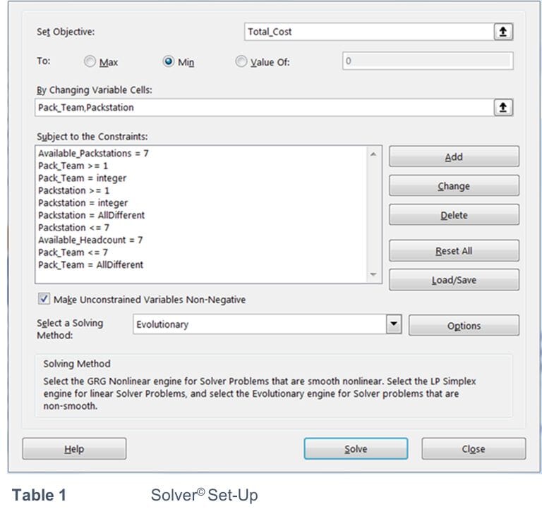
Table 1 Solver© Setup
Our solution is driven by the couple: operators and workstations. Using the input data in our source table, we can select the cells that correspond to each of the 7 workstations and employees and submit these into the By Changing Variable Cells row in the Solver© window.
Next, from the source table, we select the individual constraint cells and install each one in the Subject to the Constraints field (paying careful attention to the relations and values).
Finally, we call on the appropriate solution method. Since the structure of this problem is nonlinear our approach can be to either select a GRG (Generalised Reduced Gradient) or Evolutionary method. The latter uses a genetic algorithm and local search methods which generally return a good solution in reasonable execution time. Often, you will find that solutions returned may not be strictly best (optimal) but nonetheless, sufficiently good (feasible).
Using the drop-down menu in the Select a Solving Method field, the Evolutionary method is chosen and, after the Solve button is depressed, the solution is returned in just under one minute.
Solution
The results are displayed on the worksheet (see Table 2) and the minimum total cost is estimated to be $116k. It can be shown that this solution is consistent for seven of ten simulation runs. Here you can see the allocation decision returned as each operator is paired with a workstation / cell. This recommended configuration will secure the minimum cost to fulfill the full order quantity while accounting for discrete scrap rates and operator efficiencies.
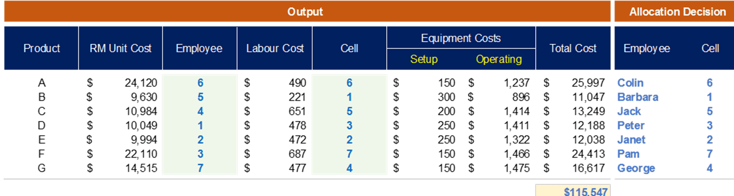
Table 2 Solution Output
The maximum cost is then evaluated by re-running the model; this is found to be around €118k. Therefore, this recommended operator-workstation pairing can potentially provide a €3k saving to produce this specific mix of orders – making this analysis worthwhile.
Detailed workings are available on request.
Next month, we shall continue our introduction to OR in the supply chain and present the Facility Location Problem. As transportation and location-specific costs are generally significant components in the supply chain, this can be addressed by locating facilities in such a way so as to minimise these combined costs.
Supply Chain Enabled